Take Home Exercise 1

Author

Hulwana

1 Overview

1.1 Getting Started

In the code chunk below, p_load() of pacman package is used to install and load the following R packages into R environment:

sf is use for importing and handling geospatial data in R,
tidyverse is mainly use for wrangling attribute data in R,
tmap will be used to prepare cartographic quality chropleth map,
spdep will be used to compute spatial weights, global and local spatial autocorrelation statistics, and
funModeling will be used for rapid Exploratory Data Analysis

pacman::p_load(sf, tidyverse, tmap, spdep, funModeling, plotly, rPackedBar)

1.2 Importing Geospatial Data

In this in-class data, two geospatial datasets will beused, they are:

geo_export
nga_admbnda_adm2_osgof_20190417

1.2.1 Importing Geospatial Data

First, we are going to import the water point geospatial data (i.e. geo_export) by using the code chunk below.

wp <- st_read(dsn = "data",
                   layer = "geo_export",
                   crs = 4326) %>%
  filter(clean_coun == "Nigeria")

Things to learn from the code chunk above:

st_read() of sf package is used to import geo_export shapefile into R environment and save the imported geospatial data into simple feature data table.
filter() of dplyr package is used to extract water point records of Nigeria.

Next, write_rds() of readr package is used to save the extracted sf data table (i.e. wp) into an output file in rds data format. The output file is called wp_nga.rds and it is saved in geodata sub-folder.

write_rds(wp, "data/wp_nga.rds")

1.2.2 Import Nigeria LGA Boundary data

Now, we are going to import the LGA boundary data into R environment by using the code chunk below.

nga <- st_read(dsn = "data",
               layer = "nga_admbnda_adm2_osgof_20190417",
               crs = 4326)

Thing to learn from the code chunk above.

st_read() of sf package is used to import nga_admbnda_adm2_osgof_20190417 shapefile into R environment and save the imported geospatial data into simple feature data table.

1.3 Data Wrangling

1.3.1 Recoding NA values into string

In the code chunk below, replace_na() is used to recode all the NA values in status_cle field into Unknown.

wp_nga <- read_rds("data/wp_nga.rds") %>%
  dplyr::mutate(status_cle = 
           replace_na(status_cle, "Unknown"))

1.3.2 EDA

In the code chunk below, freq() of funModeling package is used to display the distribution of status_cle field in wp_nga.

freq(data=wp_nga, 
     input = 'status_cle')

The above bar chart provide a brief understanding that the percentage of water-points that are functional in Nigeria is slightly less than 50%. It is crucial thus to dive deeper to determine if there are significant pattern in areas that do not have functional water-points and if the neighbouring areas can support those areas that face scarcity in water supply.

Observe that there are two categories with similar names (i.e. ‘Non-Functional due to dry season’ and ‘Non functional due to dry season’, we will standardize this by changing that later to ‘Non-Functional due to dry season’. We will also group those water-points which are marked ‘Abandoned’ with those that are grouped under ‘Abandoned/Decommissioned’.

wp_nga$status_cle[wp_nga$status_cle == "Non functional due to dry season"] <- "Non-Functional due to dry season"
wp_nga$status_cle[wp_nga$status_cle == "Abandoned"] <- "Abandoned/Decommissioned"

We rerun the above code to get the following chart

freq(data=wp_nga, 
     input = 'status_cle')

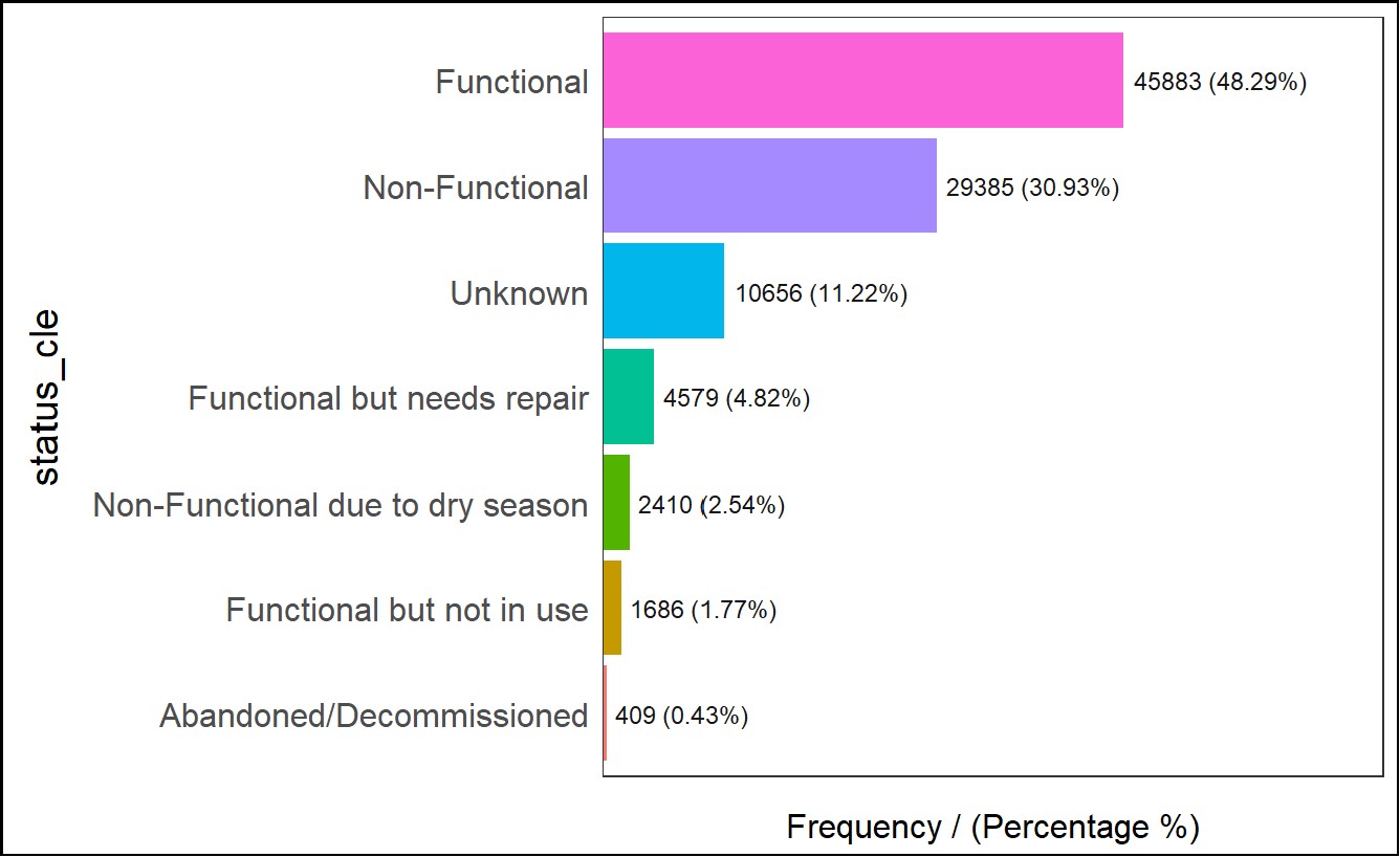
1.4 Extracting Water Point Data

In this section, we will extract the water point records by using classes in status_cle field.

1.4.1 Extracting functional water point

In the code chunk below, filter() of dplyr is used to select functional water points.

wpt_functional <- wp_nga %>%
  filter(status_cle %in%
           c("Functional", 
             "Functional but not in use",
             "Functional but needs repair"))

freq(data = wpt_functional,
     input = "status_cle")

1.4.2 Extracting non-functional water point

In the code chunk below, filter() of dplyr is used to select non-functional water points.

wpt_nonfunctional <- wp_nga %>%
  filter(status_cle %in%
           c("Abandoned/Decommissioned", 
             "Non-Functional",
             "Non-Functional due to dry season"))

freq(data=wpt_nonfunctional, 
     input = 'status_cle')

1.4.3 Extracting water point with Unknown class

In the code chunk below, filter() of dplyr is used to select water points with unknown status.

wpt_unknown <- wp_nga %>%
  filter(status_cle == "Unknown")

1.5 Performing Point-in-Polygon Count

nga_wp <- nga %>% 
  mutate(`total wpt` = lengths(
    st_intersects(nga, wp_nga))) %>%
  mutate(`wpt functional` = lengths(
    st_intersects(nga, wpt_functional))) %>%
  mutate(`wpt non-functional` = lengths(
    st_intersects(nga, wpt_nonfunctional))) %>%
  mutate(`wpt unknown` = lengths(
    st_intersects(nga, wpt_unknown)))

1.5 Saving the Analytical Data Table

nga_wp <- nga_wp %>%
  mutate(pct_functional = `wpt functional`/`total wpt`) %>%
  mutate(`pct_non-functional` = `wpt non-functional`/`total wpt`) %>%
  select(3:4, 8:10, 15:23)

Things to learn from the code chunk above:

mutate() of dplyr package is used to derive two fields namely pct_functional and pct_non-functional
to keep the file size small, select() of dplyr is used to retain only fields 3, 4, 8, 9, 10, 15, 16, 17, 18, 19, 20, 21, 22,and 23. Fields 3, 4, 8, 9, 10, 15, 16 and 17 captures the different level of geo boundaries in Nigeria. The 4 different boundaries can be seen below;
```
plot(nga_wp[,c(1,3,5,6)])
```
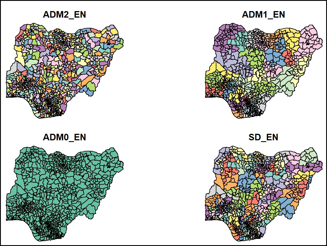
ADM2_EN: geo-mapping based on local government area (LGA)
ADM1_EN: geo-mapping based on state or federal capital territory
ADM0_EN: geo-mapping based on country
SD_EN: geo-mapping based on senatorial district

Now, that we have the tidy sf data table subsequent analysis. We will save the sf data table into rds format.

write_rds(nga_wp, "data/nga_wp.rds")

1.6 Visualizing the Spatial Distribution of Water Points

1.6.1 Visualizing based on Local Government Area (LGA) by Count

nga_wp <- read_rds("data/nga_wp.rds")
total <- qtm(nga_wp, "total wpt")
wp_functional <- qtm(nga_wp, "wpt functional")
wp_nonfunctional <- qtm(nga_wp, "wpt non-functional")
unknown <- qtm(nga_wp, "wpt unknown")

tmap_mode("view")
tmap_arrange(total, wp_functional, wp_nonfunctional, unknown, 
             asp=1, ncol=2)

Based on the above chart, we briefly observe that in terms of functional waterpoints, the north-west zone has the most functional waterpoints, whereas the number of non-functional water-points seems to be scattered all over in Nigeria.

It is interesting to note that while the district Ifelodun has a relatively higher number of functional waterpoints, it also has the highest number of non-functional waterpoints.

In terms of unknown waterpoint statuses it it mostly populated in the north-central zone of Nigeria.

1.6.2 Visualizing based on Local Government Area (LGA) by Quantile

Notice, that areas with high counts of functional waterpoints or high counts of non-functional waterpoints are rather sparse and the number of areas falling in each bucket of number scale are not evenly distributed. This might be misleading in terms of understanding the waterpoint distribution accross Nigeria and instead we will take a look at the distribution based on the quantile.

We run the code below to get the intended geo-visualization:

tmap_mode("view")
total <- tm_shape(nga_wp)+ 
  tm_fill("total wpt", style = "quantile") +
  tm_borders()

wp_functional <- tm_shape(nga_wp)+ 
  tm_fill("wpt functional", style = "quantile") +
  tm_borders()
  
wp_nonfunctional <- tm_shape(nga_wp)+ 
  tm_fill("wpt non-functional", style = "quantile") +
  tm_borders()

unknown <- tm_shape(nga_wp)+ 
  tm_fill("wpt unknown", style = "quantile") +
  tm_borders()

tmap_arrange(total, wp_functional, wp_nonfunctional, unknown, 
             asp=1, ncol=2)

Based on the above chart, we see that the above mapping is divided into many subareas. Perhaps we could visualize by a certain district or state.

1.6.3 Visualizing based on State/Federal Capital Territory by Count

To see if the number of functional and non-functional waterpoints are evenly distributed or concentrated to a specific region, we will use the ADM2_EN field to outline the broader area in Nigeria.

We will first have to aggregate the total waterpoints, total functional waterpoints, total non-functional waterpoints and total unknown waterpoints by the respective state using the following code:

nga_state <- nga_wp %>%
  group_by(ADM1_EN) %>%
  summarise(total_wp = sum(`total wpt`),
            total_functional = sum(`wpt functional`),
            total_non_functional = sum(`wpt non-functional`),
            total_unknown = sum(`wpt unknown`))

The following code chunk is executed to obtain the visualization

tmap_mode("plot")

total <- tm_shape(nga_state)+
  tm_fill("total_wp", palette="BuGn") +
  tm_borders()

wp_functional <- tm_shape(nga_state)+
  tm_fill("total_functional", palette="BuGn") +
  tm_borders()

wp_nonfunctional <- tm_shape(nga_state)+
  tm_fill("total_non_functional", palette="BuGn") +
  tm_borders()

unknown <- tm_shape(nga_state)+
  tm_fill("total_unknown", palette="BuGn") +
  tm_borders()

tmap_arrange(total, wp_functional, wp_nonfunctional, unknown,
             asp=1, ncol=2)

In contrast to plotting based on LGA, we see that for non-functional points are more spread based on the plotting via state region.

However, in terms of total waterpoints, total functional waterpoints and total unknown waterpoints have number of areas that are uniformly distributed against the number category, we will proceed to plot the distribution via quantile instead of count.

1.6.4 Visualizing based on State/Federal Capital Territory by Quantile

To visualize the distribution of waterpoints across the different state in Nigeria, we run the following code:

tmap_mode("plot")

total <- tm_shape(nga_state)+
  tm_fill("total_wp", palette="BuGn", style="quantile") +
  tm_borders()

wp_functional <- tm_shape(nga_state)+
  tm_fill("total_functional", palette="BuGn", style="quantile") +
  tm_borders()

wp_nonfunctional <- tm_shape(nga_state)+
  tm_fill("total_non_functional", palette="BuGn", style="quantile") +
  tm_borders()

unknown <- tm_shape(nga_state)+
  tm_fill("total_unknown", palette="BuGn", style="quantile") +
  tm_borders()

tmap_arrange(total, wp_functional, wp_nonfunctional, unknown,
             asp=1, ncol=2)

2 Analysis of Non-functional Water Points

2.1 Further transformation

In geospatial analytics, it is very common for us to transform the original data from geographic coordinate system to projected coordinate system. This is because geographic coordinate system is not appropriate if the analysis need to use distance or/and area measurements.

The print below reveals that the assigned coordinates system is WGS 84, the ‘World Geodetic System 1984’ which is inappropriate in our case and should be using the CRS of Nigeria with an ESPG code of either 26391, 26392, and 26303. A country’s epsg code can be obtained by referring to epsg.io.

We will use the EPSG code of 26391 in our analysis.

st_geometry(nga_wp)

Geometry set for 774 features 
Geometry type: MULTIPOLYGON
Dimension:     XY
Bounding box:  xmin: 2.668534 ymin: 4.273007 xmax: 14.67882 ymax: 13.89442
Geodetic CRS:  WGS 84
First 5 geometries:

Based on the initial dataset it is in Geodetic CRS and thus we need to reproject nga_wp to another coordinate system mathemetically using the st_transform function of the sf package, as shown by the code chunk below.

nga_wp26391 <- st_transform(nga_wp, crs = 26391)

Next, we will view the content of nga_wp26391 sf data frame as shown below.

st_geometry(nga_wp26391)

Geometry set for 774 features 
Geometry type: MULTIPOLYGON
Dimension:     XY
Bounding box:  xmin: 28879.72 ymin: 30292.37 xmax: 1343798 ymax: 1094244
Projected CRS: Minna / Nigeria West Belt
First 5 geometries:

Notice that instead of Geodetic CRS it has been changed to a Projected CRS of Minna / Nigeria West Belt.

2.2 Visualization

2.2.1 Geo Distribution of non-functional water points across Nigeria based on LGA

tmap_mode("plot")

wp_nonfunctional_count <- tm_shape(nga_wp26391) +
  tm_fill("wpt non-functional", palette="Reds") +
  tm_borders() +
  tm_layout(main.title = "Equal Interval Classification",
            legend.position = c("right", "bottom"))

wp_nonfunctional_quantile <- tm_shape(nga_wp26391) +
  tm_fill("wpt non-functional", palette="Reds", style="quantile") +
  tm_borders() +
  tm_layout(main.title = "Equal Quantile Classification ",
            legend.position = c("right", "bottom"))

tmap_arrange(wp_nonfunctional_count, wp_nonfunctional_quantile,
             asp=1, ncol=2)

2.2.2 Areas with most non-functional water points

plotly_packed_bar(nga_wp,
                  label_column = "ADM2_EN",
                  value_column = "wpt non-functional")

2.3 Computing distance based neighbours

In this section, we will derive distance-based weight matrices by using dnearneigh() of spdep package.

The function identifies neighbours of region points by Euclidean distance with a distance band with lower d1= and upper d2= bounds controlled by the bounds= argument. If unprojected coordinates are used and either specified in the coordinates object x or with x as a two column matrix and longlat=TRUE, great circle distances in km will be calculated assuming the WGS84 reference ellipsoid.

2.3.1 Obtaining the coordinate values

To get our longitude values we map the st_centroid function over the geometry column of us.bound and access the longitude value through double bracket notation [[]] and 1. This allows us to get only the longitude, which is the first value in each centroid.

longitude <- purrr::map_dbl(nga_wp$geometry, ~st_centroid(.x)[[1]])

We do the same for latitude with one key difference. We access the second value per each centroid with [[2]].

latitude <- purrr::map_dbl(nga_wp$geometry, ~st_centroid(.x)[[2]])

Now that we have latitude and longitude, we use cbind to put longitude and latitude into the same object.

coords <- cbind(longitude, latitude)

We check the first few observations to see if things are formatted correctly.

head(coords)

     longitude  latitude
[1,]  7.372450  5.113107
[2,]  7.352131  5.083219
[3,] 13.322900 13.428835
[4,]  6.847325  8.825812
[5,]  7.771541  5.022061
[6,]  8.219654  6.259845

2.3.2 Determining the cut-off distance

Firstly, we need to determine the upper limit for distance band by using the steps below:

Return a matrix with the indices of points belonging to the set of the k nearest neighbours of each other by using knearneigh() of spdep.
Convert the knn object returned by knearneigh() into a neighbours list of class nb with a list of integer vectors containing neighbour region number ids by using knn2nb().
Return the length of neighbour relationship edges by using nbdists() of spdep. The function returns in the units of the coordinates if the coordinates are projected, in km otherwise.
Remove the list structure of the returned object by using unlist().

k1 <- knn2nb(knearneigh(coords))
k1dists <- unlist(nbdists(k1, coords, longlat = TRUE))
summary(k1dists)

   Min. 1st Qu.  Median    Mean 3rd Qu.    Max. 
  2.662  12.815  20.242  22.031  27.706  71.661

The summary report shows that the largest first nearest neighbour distance is 71.66 km, so using this as the upper threshold gives certainty that all units will have at least one neighbour.

2.3.3 Computing fixed distance weight matrix

Now, we will compute the distance weight matrix by using dnearneigh() as shown in the code chunk below.

wm_d72 <- dnearneigh(coords, 0, 72, longlat = TRUE)
wm_d72

Neighbour list object:
Number of regions: 774 
Number of nonzero links: 18112 
Percentage nonzero weights: 3.023323 
Average number of links: 23.40052

Notice that the average number of links is 23, this meant that for each area the average number of neigbours based on the distance set is 23.

The neighours of each area can be displayed by executing the following code:

str(wm_d72)

2.3.3.1 Plotting fixed distance weight matrix

To visualize the links between each neighbours, we run the code chunk:

plot(nga_wp$geometry, border="lightgrey")
plot(wm_d72, coords, add=TRUE)
plot(k1, coords, add=TRUE, col="red", length=0.08)

The red lines show the links of 1st nearest neighbours and the black lines show the links of neighbours within the cut-off distance of 72km.

As we see that there are huge patches of black in the plot thus making the visualization difficult to distinguish the links between neighbours, we can plot both of them next to each other by using the code chunk below.

par(mfrow=c(1,2))
plot(nga_wp$geometry, border="lightgrey")
plot(k1, coords, add=TRUE, col="red", length=0.08, main="1st nearest neighbours")
plot(nga_wp$geometry, border="lightgrey")
plot(wm_d72, coords, add=TRUE, pch = 19, cex = 0.6, main="Distance link")

Despite the separation of plots, it is still hard to see the distinct 1st nearest nighbours links for some areas due to the close proximity. Thus, to achieve a more balance number of neighbours for each area, we will analysed based on the adaptive distance weight matrix.

2.3.4 Computing adaptive distance weight matrix

One of the characteristics of fixed distance weight matrix is that more densely settled areas (usually the urban areas) tend to have more neighbours and the less densely settled areas (usually the rural counties) tend to have lesser neighbours. Having many neighbours smoothes the neighbour relationship across more neighbours.

It is possible to control the numbers of neighbours directly using k-nearest neighbours, either accepting asymmetric neighbours or imposing symmetry as shown in the code chunk below.

knn8 <- knn2nb(knearneigh(coords, k=8))
knn8

Neighbour list object:
Number of regions: 774 
Number of nonzero links: 6192 
Percentage nonzero weights: 1.033592 
Average number of links: 8 
Non-symmetric neighbours list

Similarly, we can display the content of the matrix by using str().

str(knn8)

2.3.4.1 Plotting distance based neighbours

We can plot the weight matrix using the code chunk below.

plot(nga_wp$geometry, border="lightgrey")
plot(knn8, coords, pch = 19, cex = 0.6, add = TRUE, col = "navyblue")

2.3.5 Weights based on IDW

In this section, we will derive a spatial weight matrix based on Inversed Distance method.

First, we will compute the distances between areas by using nbdists() of spdep.

dist <- nbdists(knn8, coords, longlat = TRUE)
ids <- lapply(dist, function(x) 1/(x))

2.3.5.1 Row-standardised weights matrix

Next, we need to assign weights to each neighboring polygon. In our case, each neighboring polygon will be assigned equal weight (style=“W”). This is accomplished by assigning the fraction 1/(#ofneighbors) to each neighboring county then summing the weighted income values. While this is the most intuitive way to summaries the neighbors’ values it has one drawback in that polygons along the edges of the study area will base their lagged values on fewer polygons thus potentially over- or under-estimating the true nature of the spatial autocorrelation in the data. For this example, we’ll stick with the style=“W” option for simplicity’s sake but note that other more robust options are available, notably style=“B”.

rswm_knn8 <- nb2listw(knn8, style="W", zero.policy = TRUE)
rswm_knn8

Characteristics of weights list object:
Neighbour list object:
Number of regions: 774 
Number of nonzero links: 6192 
Percentage nonzero weights: 1.033592 
Average number of links: 8 
Non-symmetric neighbours list

Weights style: W 
Weights constants summary:
    n     nn  S0     S1       S2
W 774 599076 774 174.25 3155.344

The zero.policy=TRUE option allows for lists of non-neighbors. This should be used with caution since the user may not be aware of missing neighbors in their dataset however, a zero.policy of FALSE would return an error.

To see the weight of the first polygon’s eight neighbors type:

rswm_knn8$weights[10]

[[1]]
[1] 0.125 0.125 0.125 0.125 0.125 0.125 0.125 0.125

Each neighbor is assigned a 0.125 of the total weight. This means that when R computes the average neighboring income values, each neighbor’s income will be multiplied by 0.125 before being tallied.

Using the same method, we can also derive a row standardised distance weight matrix by using the code chunk below.

rswm_ids <- nb2listw(knn8, glist=ids, style="B", zero.policy=TRUE)
rswm_ids

Characteristics of weights list object:
Neighbour list object:
Number of regions: 774 
Number of nonzero links: 6192 
Percentage nonzero weights: 1.033592 
Average number of links: 8 
Non-symmetric neighbours list

Weights style: B 
Weights constants summary:
    n     nn       S0       S1       S2
B 774 599076 239.9499 30.58247 455.9661

rswm_ids$weights[1]

[[1]]
[1] 0.25000205 0.04660966 0.05059913 0.09046782 0.06208171 0.10747703 0.09375983
[8] 0.04799011

summary(unlist(rswm_ids$weights))

    Min.  1st Qu.   Median     Mean  3rd Qu.     Max. 
0.005364 0.019893 0.029968 0.038752 0.045623 0.375598

2.4 Application of Spatial Weight Matrix

In this section, we will examine spatial lag with row-standardized weights.

2.4.1 Spatial lag with row-standardized weights

To compute the average neighbour non-functional waterpoints also known as spatially lagged values we execute the following code using the function lag.listw() of the spdep package:

Nonfunc_lag <- lag.listw(rswm_knn8, nga_wp$`wpt non-functional`)
Nonfunc_lag[1:10]

 [1] 45.000 46.375  0.250 47.375 34.000 68.375 33.375 23.375 66.125 24.750

We can append the spatially lag non-functional waterpoint values onto nga_wp data frame by using the code chunk below.

lag.list <- list(nga_wp$ADM2_EN, lag.listw(rswm_knn8, nga_wp$`wpt non-functional`))
lag.res <- as.data.frame(lag.list)
colnames(lag.res) <- c("ADM2_EN", "lag nonFunctional wp")
nigeria_wp <- left_join(nga_wp,lag.res)

The following table shows the average neighboring number of non-functional waterpoint (stored in the Inc.lag object) for each county.

head(nigeria_wp)

Simple feature collection with 6 features and 14 fields
Geometry type: MULTIPOLYGON
Dimension:     XY
Bounding box:  xmin: 6.778522 ymin: 4.888055 xmax: 13.83477 ymax: 13.71406
Geodetic CRS:  WGS 84
    ADM2_EN ADM2_PCODE                   ADM1_EN ADM1_PCODE ADM0_EN
1 Aba North   NG001001                      Abia      NG001 Nigeria
2 Aba South   NG001002                      Abia      NG001 Nigeria
3    Abadam   NG008001                     Borno      NG008 Nigeria
4     Abaji   NG015001 Federal Capital Territory      NG015 Nigeria
5      Abak   NG003001                 Akwa Ibom      NG003 Nigeria
6 Abakaliki   NG011001                    Ebonyi      NG011 Nigeria
                      SD_EN SD_PCODE total wpt wpt functional
1                Abia South  NG00103        17              7
2                Abia South  NG00103        71             29
3               Borno North  NG00802         0              0
4 Federal Capital Territory  NG01501        57             23
5      Akwa Ibom North West  NG00302        48             23
6              Ebonyi North  NG01103       233             82
  wpt non-functional wpt unknown pct_functional pct_non-functional
1                  9           1      0.4117647          0.5294118
2                 35           7      0.4084507          0.4929577
3                  0           0            NaN                NaN
4                 34           0      0.4035088          0.5964912
5                 25           0      0.4791667          0.5208333
6                 42         109      0.3519313          0.1802575
  lag nonFunctional wp                       geometry
1               45.000 MULTIPOLYGON (((7.401109 5....
2               46.375 MULTIPOLYGON (((7.387495 5....
3                0.250 MULTIPOLYGON (((13.83477 13...
4               47.375 MULTIPOLYGON (((7.045872 9....
5               34.000 MULTIPOLYGON (((7.811244 5....
6               68.375 MULTIPOLYGON (((8.4109 6.28...

2.4.2 Comparing actual number of non-functional waterpoints and spatially lag values

Next, we will plot both the non-fucntional waterpoints and spatial lag non-fucntional waterpoints for comparison using the code chunk below.

nonf <- qtm(nigeria_wp, "wpt non-functional")
lag_nonf <- qtm(nigeria_wp, "lag nonFunctional wp")
tmap_arrange(nonf, lag_nonf, asp=1, ncol=2)

Observe that in comparison to the actual number of non-functional waterpoint found in area shown on the left chart, the spatially lag values shows that there quite a significant number of areas that have medium to high amount of non-functional waterpoints in their neighbouring areas. This might posed as a possible area of concern as when there is a shortage of water experienced by their neighbours, it might indirectly affect the amount of water available for their own areas as well.

3 Global Spatial Autocorrelation

We will now compute global spatial autocorrelation statistics and to perform spatial complete randomness test for global spatial autocorrelation.

3.1 Global Spatial Autocorrelation: Moran’s I

3.1.1 Moran’s I test

We will perform Moran’s I statistics testing by using moran.test() of spdep using the earlier computed weight matrix of rswm_knn8.

moran.test(nga_wp$'wpt non-functional', 
           listw = rswm_knn8, 
           zero.policy = TRUE, 
           na.action=na.omit)


    Moran I test under randomisation

data:  nga_wp$"wpt non-functional"  
weights: rswm_knn8    

Moran I statistic standard deviate = 22.673, p-value < 2.2e-16
alternative hypothesis: greater
sample estimates:
Moran I statistic       Expectation          Variance 
     0.3822703126     -0.0012936611      0.0002861956

3.1.2 Computing Monte Carlo Moran’s I

The code chunk below performs permutation test for Moran’s I statistic by using moran.mc() of spdep. A total of 1000 simulation will be performed. We indicate the nsim to be 999 as it starts with 0 for the first observation.

set.seed(1234)
monteM<- moran.mc(nga_wp$'wpt non-functional', 
                listw=rswm_knn8, 
                nsim=999, 
                zero.policy = TRUE, 
                na.action=na.omit)
monteM


    Monte-Carlo simulation of Moran I

data:  nga_wp$"wpt non-functional" 
weights: rswm_knn8  
number of simulations + 1: 1000 

statistic = 0.38227, observed rank = 1000, p-value = 0.001
alternative hypothesis: greater

3.1.3 Visualizing Monte Carlo Moran’s I

It is always a good practice for us the examine the simulated Moran’s I test statistics in greater detail. This can be achieved by plotting the distribution of the statistical values as a histogram by using the code chunk below.

In the code chunk below hist() and abline() of R Graphics are used.

mean(monteM$res[1:999])

[1] -0.000628295

var(monteM$res[1:999])

[1] 0.0002988427

summary(monteM$res[1:999])

      Min.    1st Qu.     Median       Mean    3rd Qu.       Max. 
-0.0570637 -0.0128308 -0.0011785 -0.0006283  0.0106868  0.0645272

hist(monteM$res, 
     freq=TRUE, 
     breaks=50, 
     xlab="Simulated Moran's I")
abline(v=0, 
       col="red")

3.2 Global Spatial Autocorrelation: Geary’s

In this section, you will learn how to perform Geary’s c statistics testing by using appropriate functions of spdep package.

3.2.1 Geary’s C test

The code chunk below performs Geary’s C test for spatial autocorrelation by using geary.test() of spdep.

geary.test(nga_wp$'wpt non-functional', listw=rswm_knn8)


    Geary C test under randomisation

data:  nga_wp$"wpt non-functional" 
weights: rswm_knn8 

Geary C statistic standard deviate = 19.315, p-value < 2.2e-16
alternative hypothesis: Expectation greater than statistic
sample estimates:
Geary C statistic       Expectation          Variance 
     0.6066280275      1.0000000000      0.0004147634

3.2.2 Computing Monte Carlo Geary’s C

The code chunk below performs Geary’s C test for spatial autocorrelation by using geary.test() of spdep.

set.seed(1234)
monteC <- geary.mc(nga_wp$'wpt non-functional', 
                listw=rswm_knn8, 
                nsim=999)
monteC


    Monte-Carlo simulation of Geary C

data:  nga_wp$"wpt non-functional" 
weights: rswm_knn8 
number of simulations + 1: 1000 

statistic = 0.60663, observed rank = 1, p-value = 0.001
alternative hypothesis: greater

3.2.3 Visualizing the Monte Carlo Geary’s C

Next, we will plot a histogram to reveal the distribution of the simulated values by using the code chunk below.

mean(monteC$res[1:999])

[1] 0.9991838

var(monteC$res[1:999])

[1] 0.0004175843

summary(monteC$res[1:999])

   Min. 1st Qu.  Median    Mean 3rd Qu.    Max. 
 0.9276  0.9859  0.9996  0.9992  1.0132  1.0699

hist(monteC$res, freq=TRUE, breaks=50, xlab="Simulated Geary c")
abline(v=1, col="red")

3.3 Spatial Correlogram

Spatial correlograms are great to examine patterns of spatial autocorrelation in your data or model residuals. They show how correlated are pairs of spatial observations when you increase the distance (lag) between them - they are plots of some index of autocorrelation (Moran’s I or Geary’s c) against distance.Although correlograms are not as fundamental as variograms (a keystone concept of geostatistics), they are very useful as an exploratory and descriptive tool. For this purpose they actually provide richer information than variograms.

3.3.1 Compute Moran’s I correlogram

In the code chunk below, sp.correlogram() of spdep package is used to compute a 6-lag spatial correlogram of non-functional waterpoints. The global spatial autocorrelation used in Moran’s I. The plot() of base Graph is then used to plot the output.

MI_corr <- sp.correlogram(knn8, 
                          nga_wp$'wpt non-functional', 
                          order=6, 
                          method="I", 
                          style="W")
plot(MI_corr)

By plotting the output might not allow us to provide complete interpretation. This is because not all autocorrelation values are statistically significant. Hence, it is important for us to examine the full analysis report by printing out the analysis results as in the code chunk below.

print(MI_corr)

Spatial correlogram for nga_wp$"wpt non-functional" 
method: Moran's I
           estimate expectation    variance standard deviate Pr(I) two sided
1 (774)  3.8227e-01 -1.2937e-03  2.8620e-04          22.6729       < 2.2e-16
2 (774)  2.4930e-01 -1.2937e-03  1.4431e-04          20.8602       < 2.2e-16
3 (774)  1.7705e-01 -1.2937e-03  9.8425e-05          17.9768       < 2.2e-16
4 (774)  1.1632e-01 -1.2937e-03  7.2941e-05          13.7707       < 2.2e-16
5 (774)  7.4244e-02 -1.2937e-03  5.7162e-05           9.9910       < 2.2e-16
6 (774)  3.3259e-02 -1.2937e-03  4.7571e-05           5.0096       5.453e-07
           
1 (774) ***
2 (774) ***
3 (774) ***
4 (774) ***
5 (774) ***
6 (774) ***
---
Signif. codes:  0 '***' 0.001 '**' 0.01 '*' 0.05 '.' 0.1 ' ' 1

3.3.2 Compute Geary’s C correlogram and plot

GC_corr <- sp.correlogram(knn8, 
                          nga_wp$'wpt non-functional', 
                          order=6, 
                          method="C", 
                          style="W")
plot(GC_corr)

Similar to the previous step, we will print out the analysis report by using the code chunk below.

print(GC_corr)

Spatial correlogram for nga_wp$"wpt non-functional" 
method: Geary's C
          estimate expectation   variance standard deviate Pr(I) two sided    
1 (774) 0.60662803  1.00000000 0.00041476         -19.3154       < 2.2e-16 ***
2 (774) 0.74002024  1.00000000 0.00030920         -14.7849       < 2.2e-16 ***
3 (774) 0.83031948  1.00000000 0.00031509          -9.5590       < 2.2e-16 ***
4 (774) 0.90248528  1.00000000 0.00026763          -5.9608        2.51e-09 ***
5 (774) 0.94830963  1.00000000 0.00024618          -3.2945       0.0009861 ***
6 (774) 0.97289919  1.00000000 0.00024566          -1.7291       0.0837962 .  
---
Signif. codes:  0 '***' 0.001 '**' 0.01 '*' 0.05 '.' 0.1 ' ' 1

4 Cluster and Outlier Analysis

4.1 Computing local Moran’s I

To compute local Moran’s I, the localmoran() function of spdep will be used. It computes Ii values, given a set of zi values and a listw object providing neighbour weighting information for the polygon associated with the zi values.

fips <- order(nga_wp$ADM2_EN)
localMI <- localmoran(nga_wp$`wpt non-functional`, rswm_knn8)
head(localMI)

            Ii          E.Ii       Var.Ii       Z.Ii Pr(z != E(Ii))
1 -0.080696263 -9.995243e-04 9.573134e-02 -0.2575808    0.796730455
2 -0.022923567 -4.092463e-05 3.923396e-03 -0.3653214    0.714871500
3  1.250637751 -1.627684e-03 1.557965e-01  3.1726160    0.001510722
4 -0.031922684 -5.427505e-05 5.203215e-03 -0.4417988    0.658634818
5  0.091666434 -2.590965e-04 2.483385e-02  0.5833297    0.559671349
6  0.007875149 -1.538445e-07 1.474949e-05  2.0505897    0.040306916

localmoran() function returns a matrix of values whose columns are:

Ii: the local Moran’s I statistics
E.Ii: the expectation of local moran statistic under the randomisation hypothesis
Var.Ii: the variance of local moran statistic under the randomisation hypothesis
Z.Ii:the standard deviate of local moran statistic
Pr(): the p-value of local moran statistic

4.1.1 Mapping the local Moran’s I

Before mapping the local Moran’s I map, it is wise to append the local Moran’s I dataframe (i.e. localMI) onto nga_wp SpatialPolygonDataFrame. The code chunks below can be used to perform the task. The out SpatialPolygonDataFrame is called nga_wp.localMI.

nga_wp.localMI <- cbind(nga_wp,localMI) %>%
  rename(Pr.Ii = Pr.z....E.Ii..)

4.1.2 Plotting local Moran’s I values

Using choropleth mapping functions of tmap package, we can plot the local Moran’s I values by using the code chinks below.

tm_shape(nga_wp.localMI) +
  tm_fill(col = "Ii", 
          style = "pretty",
          palette = "RdBu",
          title = "local moran statistics") +
  tm_borders(alpha = 0.5)

4.1.3 Plotting local Moran’s I p-values

The choropleth shows there is evidence for both positive and negative Ii values. However, it is useful to consider the p-values for each of these values, as consider above.

The code chunks below produce a choropleth map of Moran’s I p-values by using functions of tmap package.

tm_shape(nga_wp.localMI) +
  tm_fill(col = "Pr.Ii", 
          breaks=c(-Inf, 0.001, 0.01, 0.05, 0.1, Inf),
          palette="-Blues", 
          title = "local Moran's I p-values") +
  tm_borders(alpha = 0.5)

4.1.4 Plotting both geo-visualizations

For effective interpretation, it is better to plot both the local Moran’s I values map and its corresponding p-values map next to each other.

The code chunk below will be used to create such visualisation.

localMI.map <- tm_shape(nga_wp.localMI) +
  tm_fill(col = "Ii", 
          style = "pretty", 
          title = "local moran statistics") +
  tm_borders(alpha = 0.5) +
    tm_layout(main.title = "Local Moran's I Statistics ",
            legend.position = c("right", "bottom"))

pvalue.map <- tm_shape(nga_wp.localMI) +
  tm_fill(col = "Pr.Ii", 
          breaks=c(-Inf, 0.001, 0.01, 0.05, 0.1, Inf),
          palette="-Blues", 
          title = "local Moran's I p-values") +
  tm_borders(alpha = 0.5) + 
      tm_layout(main.title = "Local Moran's I p-values ",
            legend.position = c("right", "bottom"))

tmap_arrange(localMI.map, pvalue.map, asp=1, ncol=2)

4.2 Creating a LISA Cluster Map

The LISA Cluster Map shows the significant locations color coded by type of spatial autocorrelation. The first step before we can generate the LISA cluster map is to plot the Moran scatterplot.

4.2.1 Plotting Moran scatterplot

The Moran scatterplot is an illustration of the relationship between the values of the chosen attribute at each location and the average value of the same attribute at neighboring location by using moran.plot() of spdep.

nci <- moran.plot(nga_wp$`wpt non-functional`, rswm_knn8,
                  labels=as.character(nga_wp$ADM2_EN), 
                  xlab="Non-functional waterpoints", 
                  ylab="Spatially Lag non-functional waterpoints")

Notice that the plot is split in 4 quadrants. The top right corner belongs to areas that have high number of non-functional waterpoints and are surrounded by other areas that have the average level of non-functional waterpoints. This are the high-high locations in the lesson slide.

4.2.2 Plotting Moran scatterplot with standardised variable

First we will use scale() to centers and scales the variable. Here centering is done by subtracting the mean (omitting NAs) the corresponding columns, and scaling is done by dividing the (centered) variable by their standard deviations.

nga_wp$Z.nf <- scale(nga_wp$`wpt non-functional`) %>% 
  as.vector

The as.vector() added to the end is to make sure that the data type we get out of this is a vector, that map neatly into out dataframe.

Now, we are ready to plot the Moran scatterplot again by using the code chunk below.

nci2 <- moran.plot(nga_wp$Z.nf, rswm_knn8,
                   labels=as.character(nga_wp$ADM2_EN),
                   xlab="Z-non-functional Waterpoints", 
                   ylab="Spatially Lag Z-non-functional Waterpoints")

4.3 Preparing LISA MAP Classes

The code chunks below show the steps to prepare a LISA cluster map.

quadrant <- vector(mode="numeric",length=nrow(localMI))

Next, derives the spatially lagged variable of interest (i.e. non-functional waterpoints) and centers the spatially lagged variable around its mean.

nga_wp$lag_nf <- lag.listw(rswm_knn8, nga_wp$`wpt non-functional`)
DV <- nga_wp$lag_nf - mean(nga_wp$lag_nf)

This is follow by centering the local Moran’s around the mean.

LM_I <- localMI[,1] - mean(localMI[,1])

Next, we will set a statistical significance level for the local Moran.

signif <- 0.05

These four command lines define the low-low (1), low-high (2), high-low (3) and high-high (4) categories.

quadrant[DV <0 & LM_I>0] <- 1
quadrant[DV >0 & LM_I<0] <- 2
quadrant[DV <0 & LM_I<0] <- 3  
quadrant[DV >0 & LM_I>0] <- 4

Lastly, places non-significant Moran in the category 0.

quadrant[localMI[,5]>signif] <- 0

4.4 Plotting LISA Map

Now, we can build the LISA map by using the code chunks below.

nga_wp.localMI$quadrant <- quadrant
colors <- c("#ffffff", "#2c7bb6", "#abd9e9", "#fdae61", "#d7191c")
clusters <- c("insignificant", "low-low", "low-high", "high-low", "high-high")

tm_shape(nga_wp.localMI) +
  tm_fill(col = "quadrant", 
          style = "cat", 
          palette = colors[c(sort(unique(quadrant)))+1], 
          labels = clusters[c(sort(unique(quadrant)))+1],
          popup.vars = c("")) +
  tm_view(set.zoom.limits = c(11,17)) +
  tm_borders(alpha=0.5)

For effective interpretation, it is better to plot both the local Moran’s I values map and its corresponding p-values map next to each other.

The code chunk below will be used to create such visualization.

non_func_wp <- qtm(nga_wp, "wpt non-functional")

nga_wp.localMI$quadrant <- quadrant
colors <- c("#ffffff", "#2c7bb6", "#abd9e9", "#fdae61", "#d7191c")
clusters <- c("insignificant", "low-low", "low-high", "high-low", "high-high")

LISAmap <- tm_shape(nga_wp.localMI) +
  tm_fill(col = "quadrant", 
          style = "cat", 
          palette = colors[c(sort(unique(quadrant)))+1], 
          labels = clusters[c(sort(unique(quadrant)))+1],
          popup.vars = c("")) +
  tm_view(set.zoom.limits = c(11,17)) +
  tm_borders(alpha=0.5)

tmap_arrange(non_func_wp, LISAmap, 
             asp=1, ncol=2)

5 Hot Spot and Cold Spot Area Analysis

Beside detecting cluster and outliers, localised spatial statistics can be also used to detect hot spot and/or cold spot areas.

The term ‘hot spot’ has been used generically across disciplines to describe a region or value that is higher relative to its surroundings (Lepers et al 2005, Aben et al 2012, Isobe et al 2015).

5.1 Getis and Ord’s G-Statistics

The analysis consists of three parts:

Deriving spatial weight matrix
Computing Gi statistics
Mapping Gi statistics

5.1.1 Deriving distance-based weight matrix

First, we need to define a new set of neighbours. Whist the spatial autocorrelation considered units which shared borders, for Getis-Ord we are defining neighbours based on distance.

There are two type of distance-based proximity matrix, they are:

fixed distance weight matrix; and (see section 2.3.3)
adaptive distance weight matrix. (see section 2.3.4)

5.1.1.1 Fixed distance weight matrix

Continued form section 2.3.3, we use nb2listw() to convert the nb object into spatial weights object.

wm72_lw <- nb2listw(wm_d72, style = 'B')
summary(wm72_lw)

Characteristics of weights list object:
Neighbour list object:
Number of regions: 774 
Number of nonzero links: 18112 
Percentage nonzero weights: 3.023323 
Average number of links: 23.40052 
Link number distribution:

 1  2  3  4  5  6  7  8  9 10 11 12 13 14 15 16 17 18 19 20 21 22 23 24 25 26 
 5  8 12 21 32 35 33 35 28 36 25 21 19 23 16 14 10 13 15 17 16 11 13 10  6 12 
27 28 29 30 31 32 33 34 35 36 37 38 39 40 41 42 43 44 45 46 47 48 49 50 51 52 
12  5 16 13 12  7  9  9 12  7 12 15 13  9 10  4  5  4  7  8  8  8  6  5  3  2 
53 54 55 56 57 58 59 60 61 62 63 64 65 67 68 70 
 3  4  5  3  6  5  2  6  4  8  8  4  4  3  1  1 
5 least connected regions:
90 112 123 237 670 with 1 link
1 most connected region:
585 with 70 links

Weights style: B 
Weights constants summary:
    n     nn    S0    S1      S2
B 774 599076 18112 36224 2614072

5.1.1.2 Adaptive distance weight matrix

Continued form section 2.3.4, we use nb2listw() to convert the nb object into spatial weights object.

knn_lw <- nb2listw(knn8, style = 'B')
summary(knn_lw)

Characteristics of weights list object:
Neighbour list object:
Number of regions: 774 
Number of nonzero links: 6192 
Percentage nonzero weights: 1.033592 
Average number of links: 8 
Non-symmetric neighbours list
Link number distribution:

  8 
774 
774 least connected regions:
1 2 3 4 5 6 7 8 9 10 11 12 13 14 15 16 17 18 19 20 21 22 23 24 25 26 27 28 29 30 31 32 33 34 35 36 37 38 39 40 41 42 43 44 45 46 47 48 49 50 51 52 53 54 55 56 57 58 59 60 61 62 63 64 65 66 67 68 69 70 71 72 73 74 75 76 77 78 79 80 81 82 83 84 85 86 87 88 89 90 91 92 93 94 95 96 97 98 99 100 101 102 103 104 105 106 107 108 109 110 111 112 113 114 115 116 117 118 119 120 121 122 123 124 125 126 127 128 129 130 131 132 133 134 135 136 137 138 139 140 141 142 143 144 145 146 147 148 149 150 151 152 153 154 155 156 157 158 159 160 161 162 163 164 165 166 167 168 169 170 171 172 173 174 175 176 177 178 179 180 181 182 183 184 185 186 187 188 189 190 191 192 193 194 195 196 197 198 199 200 201 202 203 204 205 206 207 208 209 210 211 212 213 214 215 216 217 218 219 220 221 222 223 224 225 226 227 228 229 230 231 232 233 234 235 236 237 238 239 240 241 242 243 244 245 246 247 248 249 250 251 252 253 254 255 256 257 258 259 260 261 262 263 264 265 266 267 268 269 270 271 272 273 274 275 276 277 278 279 280 281 282 283 284 285 286 287 288 289 290 291 292 293 294 295 296 297 298 299 300 301 302 303 304 305 306 307 308 309 310 311 312 313 314 315 316 317 318 319 320 321 322 323 324 325 326 327 328 329 330 331 332 333 334 335 336 337 338 339 340 341 342 343 344 345 346 347 348 349 350 351 352 353 354 355 356 357 358 359 360 361 362 363 364 365 366 367 368 369 370 371 372 373 374 375 376 377 378 379 380 381 382 383 384 385 386 387 388 389 390 391 392 393 394 395 396 397 398 399 400 401 402 403 404 405 406 407 408 409 410 411 412 413 414 415 416 417 418 419 420 421 422 423 424 425 426 427 428 429 430 431 432 433 434 435 436 437 438 439 440 441 442 443 444 445 446 447 448 449 450 451 452 453 454 455 456 457 458 459 460 461 462 463 464 465 466 467 468 469 470 471 472 473 474 475 476 477 478 479 480 481 482 483 484 485 486 487 488 489 490 491 492 493 494 495 496 497 498 499 500 501 502 503 504 505 506 507 508 509 510 511 512 513 514 515 516 517 518 519 520 521 522 523 524 525 526 527 528 529 530 531 532 533 534 535 536 537 538 539 540 541 542 543 544 545 546 547 548 549 550 551 552 553 554 555 556 557 558 559 560 561 562 563 564 565 566 567 568 569 570 571 572 573 574 575 576 577 578 579 580 581 582 583 584 585 586 587 588 589 590 591 592 593 594 595 596 597 598 599 600 601 602 603 604 605 606 607 608 609 610 611 612 613 614 615 616 617 618 619 620 621 622 623 624 625 626 627 628 629 630 631 632 633 634 635 636 637 638 639 640 641 642 643 644 645 646 647 648 649 650 651 652 653 654 655 656 657 658 659 660 661 662 663 664 665 666 667 668 669 670 671 672 673 674 675 676 677 678 679 680 681 682 683 684 685 686 687 688 689 690 691 692 693 694 695 696 697 698 699 700 701 702 703 704 705 706 707 708 709 710 711 712 713 714 715 716 717 718 719 720 721 722 723 724 725 726 727 728 729 730 731 732 733 734 735 736 737 738 739 740 741 742 743 744 745 746 747 748 749 750 751 752 753 754 755 756 757 758 759 760 761 762 763 764 765 766 767 768 769 770 771 772 773 774 with 8 links
774 most connected regions:
1 2 3 4 5 6 7 8 9 10 11 12 13 14 15 16 17 18 19 20 21 22 23 24 25 26 27 28 29 30 31 32 33 34 35 36 37 38 39 40 41 42 43 44 45 46 47 48 49 50 51 52 53 54 55 56 57 58 59 60 61 62 63 64 65 66 67 68 69 70 71 72 73 74 75 76 77 78 79 80 81 82 83 84 85 86 87 88 89 90 91 92 93 94 95 96 97 98 99 100 101 102 103 104 105 106 107 108 109 110 111 112 113 114 115 116 117 118 119 120 121 122 123 124 125 126 127 128 129 130 131 132 133 134 135 136 137 138 139 140 141 142 143 144 145 146 147 148 149 150 151 152 153 154 155 156 157 158 159 160 161 162 163 164 165 166 167 168 169 170 171 172 173 174 175 176 177 178 179 180 181 182 183 184 185 186 187 188 189 190 191 192 193 194 195 196 197 198 199 200 201 202 203 204 205 206 207 208 209 210 211 212 213 214 215 216 217 218 219 220 221 222 223 224 225 226 227 228 229 230 231 232 233 234 235 236 237 238 239 240 241 242 243 244 245 246 247 248 249 250 251 252 253 254 255 256 257 258 259 260 261 262 263 264 265 266 267 268 269 270 271 272 273 274 275 276 277 278 279 280 281 282 283 284 285 286 287 288 289 290 291 292 293 294 295 296 297 298 299 300 301 302 303 304 305 306 307 308 309 310 311 312 313 314 315 316 317 318 319 320 321 322 323 324 325 326 327 328 329 330 331 332 333 334 335 336 337 338 339 340 341 342 343 344 345 346 347 348 349 350 351 352 353 354 355 356 357 358 359 360 361 362 363 364 365 366 367 368 369 370 371 372 373 374 375 376 377 378 379 380 381 382 383 384 385 386 387 388 389 390 391 392 393 394 395 396 397 398 399 400 401 402 403 404 405 406 407 408 409 410 411 412 413 414 415 416 417 418 419 420 421 422 423 424 425 426 427 428 429 430 431 432 433 434 435 436 437 438 439 440 441 442 443 444 445 446 447 448 449 450 451 452 453 454 455 456 457 458 459 460 461 462 463 464 465 466 467 468 469 470 471 472 473 474 475 476 477 478 479 480 481 482 483 484 485 486 487 488 489 490 491 492 493 494 495 496 497 498 499 500 501 502 503 504 505 506 507 508 509 510 511 512 513 514 515 516 517 518 519 520 521 522 523 524 525 526 527 528 529 530 531 532 533 534 535 536 537 538 539 540 541 542 543 544 545 546 547 548 549 550 551 552 553 554 555 556 557 558 559 560 561 562 563 564 565 566 567 568 569 570 571 572 573 574 575 576 577 578 579 580 581 582 583 584 585 586 587 588 589 590 591 592 593 594 595 596 597 598 599 600 601 602 603 604 605 606 607 608 609 610 611 612 613 614 615 616 617 618 619 620 621 622 623 624 625 626 627 628 629 630 631 632 633 634 635 636 637 638 639 640 641 642 643 644 645 646 647 648 649 650 651 652 653 654 655 656 657 658 659 660 661 662 663 664 665 666 667 668 669 670 671 672 673 674 675 676 677 678 679 680 681 682 683 684 685 686 687 688 689 690 691 692 693 694 695 696 697 698 699 700 701 702 703 704 705 706 707 708 709 710 711 712 713 714 715 716 717 718 719 720 721 722 723 724 725 726 727 728 729 730 731 732 733 734 735 736 737 738 739 740 741 742 743 744 745 746 747 748 749 750 751 752 753 754 755 756 757 758 759 760 761 762 763 764 765 766 767 768 769 770 771 772 773 774 with 8 links

Weights style: B 
Weights constants summary:
    n     nn   S0    S1     S2
B 774 599076 6192 11152 201942

5.2 Computing Gi Statistics

5.2.1 Gi Statistics using fixed distance

fips <- order(nga_wp$ADM2_EN)
gi.fixed <- localG(nga_wp$`wpt non-functional`, wm72_lw)

nga_wp.gi <- cbind(nga_wp, as.matrix(gi.fixed)) %>%
  rename(gstat_fixed = as.matrix.gi.fixed.)

5.2.2 Mapping Gi values with fixed distance weights

nf_wpt <- qtm(nga_wp, "wpt non-functional")

Gimap <-tm_shape(nga_wp.gi) +
  tm_fill(col = "gstat_fixed", 
          style = "pretty",
          palette="-RdBu",
          title = "local Gi") +
  tm_borders(alpha = 0.5)

tmap_arrange(nf_wpt, Gimap, asp=1, ncol=2)

5.2.3 Gi Statistics using adaptive distance

fips <- order(nga_wp$ADM2_EN)
gi.adaptive <- localG(nga_wp$`wpt non-functional`, knn_lw)
nga_wp.gi <- cbind(nga_wp, as.matrix(gi.adaptive)) %>%
  rename(gstat_adaptive = as.matrix.gi.adaptive.)

5.2.4 Mapping Gi values with adaptive distance weights

nf_wpt <- qtm(nga_wp, "wpt non-functional")

Gimap <-tm_shape(nga_wp.gi) +
  tm_fill(col = "gstat_adaptive", 
          style = "pretty",
          palette="-RdBu",
          title = "local Gi") +
  tm_borders(alpha = 0.5)

tmap_arrange(nf_wpt, Gimap, asp=1, ncol=2)